Case Study: Feedforward AGV Magnetic Guidance

Abstract

Magnetic tape guidance is a reliable method for industrial material flow, but traditional sensors provide only lateral position, leading to delayed responses to curvature and disturbances. The Naviq MTS160 sensor augments this with the tape's local heading angle. We incorporate this angle as a steering feedforward term in a differential-drive controller and evaluate it on a compact automated guided vehicle (AGV) testbed navigating an office track with merges, forks, and a charging spur. A minimal marker scheme—using left/right routing markers, a navicode coded marer to trigger slowdown and precise stopping, and a magnetic point marker for final docking—supports repeatable experiments and accurate charger alignment. Compared to a position-only baseline tuned for maximum stable gains, the position+angle controller achieves lower tracking error (mean absolute error reduced by 83%), requires smaller proportional gains, and shows reduced sensitivity to mechanical slack or compliance.

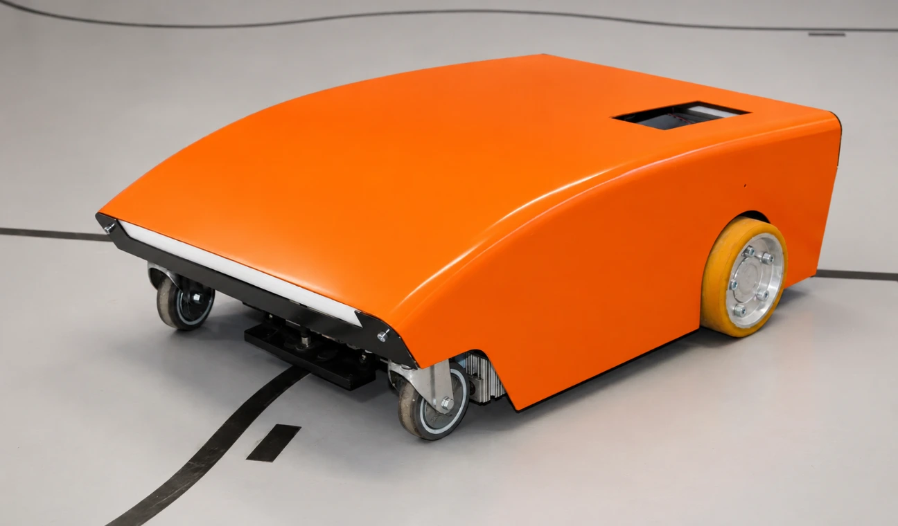
Figure 1: Compact differential-drive AGV used for experiments, equipped with the MTS160 magnetic guide sensor and controlled via a Raspberry Pi over CAN.

1. Introduction

Tape-guided AGVs are widely used in industrial material handling for their predictable paths, low infrastructure costs, and ease of reconfiguration. However, conventional sensors detect only lateral position, often requiring high feedback gains to manage curves and disturbances, which can lead to instability.

The NaviQ MTS160 addresses this by measuring both lateral offset and the tape's local heading angle. By using the angle as a feedforward steering term, the controller anticipates path changes, reducing reliance on feedback and enhancing stability.

This case study details our evaluation, including the AGV platform, track and marker design, sensing and control methods, and experimental results. We also discuss implications for commissioning, robustness, and docking precision.

2. System Overview

2.1 Hardware Platform

The testbed is a compact differential-drive AGV with two independently driven rear wheels and a front free caster. Each wheel operates under closed-loop speed control via its motor controller. A Raspberry Pi manages the system, interfacing with the MTS160 sensor and motor controllers over CAN. The control loop, written in Python, processes perception, navigation, and steering at 100 Hz.

2.2 Sensor Capabilities

The MTS160 detects magnetic tape and reports two candidate lines (left and right), each with lateral offset and heading angle relative to the sensor frame. In straight sections, candidates align; at forks and merges, they diverge, allowing the controller to select based on markers (detailed in Section 3).

3. Track Layout and Marker-Based Navigation

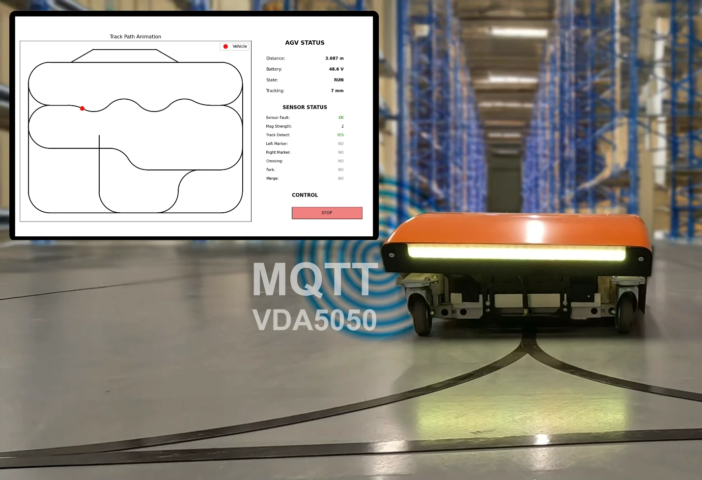
Experiments use a closed office track with merges, forks, crossings, and a charging dock to test the controller under varying curvatures and transitions.

Figure 3: Base track layout with direction markers, merges/forks, and charging spur.

Routing employs a simple, field-reconfigurable marker system:

Routing Markers: Placed before forks, these indicate left or right path selection.
Navicode: A short magnetic pattern before the docking segment, encoded using a sequence of left and right magnetic tape. The MTS160 decodes and reports it to the controller.
Docking Trigger: A specific navicode value prompts speed reduction and arms point-marker detection.
Point Marker: On the spur, this provides millimeter-level longitudinal positioning for precise stopping at the charger.

Figure 4 shows the AGV's trajectory along the track, as it follows the left/right path selection of markers. This system is easy to visualize and update in the field, and is extremely flexible.

Figure 4: AGV trajectory along the base track (split for clarity).

4. Sensing and Closed-Loop Control

Figure 5: Kinematic reference for the differential-drive AGV.

To convert sensor readings into motor commands, we derive kinematics at the sensor location. The goal is to control the speed and steering angle at the sensor, then translate these into wheel speeds.

The sensor is mounted distance \(L\) ahead of the axle; wheel seperation is \(B\); wheel radius is \(r\). Velocity at the sensor has magnitude \(V_s\) and heading \(\theta\) relative to the AGV's forward direction axis.

Rigid-body kinematics yield:

V_b = V \cos\theta, \quad \omega_b = \frac{V \sin\theta}{L}

Where \(V_b\) is axle forward velocity and \(\omega_b\) is yaw rate.

Wheel speeds are then defined as:

V_l = V_b - \frac{B}{2}\,\omega_b, \quad V_r = V_b + \frac{B}{2}\,\omega_b

Wheel angular velocities relate to linear speeds by:

\omega_l = \frac{V_l}{r}, \quad \omega_r = \frac{V_r}{r}

From which we finally derive the full kinematic relationship, linking the velocity and steering angle to wheel speeds:

\omega_l(V,\theta) = \frac{V \cos\theta}{r} - \frac{B V \sin\theta}{2 L r}

\omega_r(V,\theta) = \frac{V \cos\theta}{r} + \frac{B V \sin\theta}{2 L r}

The next step is to determine the control law, based on the sensor track measurements of lateral position \(x\) and track angle \(\theta_{\text{track}}\) (tape angle relative to the AGV's forward axis).

We propose a simple proportional controller with feedforward to compute a steering angle command \(\theta_{\text{ctrl}}\):

\theta_{\text{ctrl}} = K_p\, x + \theta_{\text{track}} \quad (5)

We then compute wheel speeds using the kinematic equations above, substituting \(\theta_{\text{ctrl}}\) for \(\theta\). The velocity \(V\) set by the navigation layer. In our experiments, we use a constant nominal speed of \(V = 0.5\) m/s, except when approaching the docking segment.

5. Experimental Setup

We compare two controllers at nominal speed V=0.5 m/s:

Position-Only: Tuned with maximum stable Kp=10 (no oscillations).
Position+Angle: Uses reduced Kp=1.5.

Multiple runs traverse the track once. Lateral error is logged at 100 Hz. We record the full trajectory of the AGV along the track, except for the final docking sequence.

6. Results and Discussion

Figure 6 compares lateral error time series over a curved segment. The position+angle controller shows smaller transients and tighter tracking, particularly at curvature entry.

Figure 6: Lateral error time series over a representative segment: position-only vs. position+angle.

Figure 7 quantifies absolute error near a marker: position+angle reduces mean absolute error from 15 mm to 9 mm (40% improvement) and halves the 95th percentile (from 30 mm to 15 mm), indicating fewer large deviations.

Figure 7: Absolute lateral error distribution in a representative region.

The angle feedforward shifts control from reactive to anticipatory, lowering feedback demands and tuning time. Lower gains reduce sensitivity to noise, backlash, and irregularities, improving stability at merges/forks.

For integrators, this enables faster commissioning and adaptability to payload/wear changes. Docking achieves <5 mm alignment in 95% of trials via point markers. Limitations include sensor reliance on clean tape (potential issues in dusty environments) and untested scaling to high-speed/large AGVs.

7. Conclusion

Integrating tape angle as steering feedforward enhances magnetic guidance simplicity and performance. On our testbed, the MTS160-based controller delivers tighter tracking, milder gains, and greater robustness. Paired with minimal markers and NaviCode logic, it provides a practical, maintainable solution for industrial AGV deployments.